How to explain gradient descent in a university exam
Gradient descent is an iterative optimisation algorithm used in machine learning to find the local minimum of a differentiable cost function. It works by calculating the gradient of the error with respect to the model parameters, then updating those parameters in the opposite direction of the gradient. This step-by-step process continues until the algorithm reaches the lowest possible error, allowing the mathematical model to make accurate predictions.
When you sit down in the exam hall, you will almost certainly face a question asking you to define this mathematical concept or apply it to a simple regression problem. Examiners do not just want you to regurgitate a textbook formula. They are looking for evidence that you understand the physical intuition of the mathematics. You need to show you know exactly what the gradient represents, why we move against it, and how the learning rate controls the entire process. Let us break down the exact components you need to master to secure full marks on these university questions.
The core intuition and the cost function
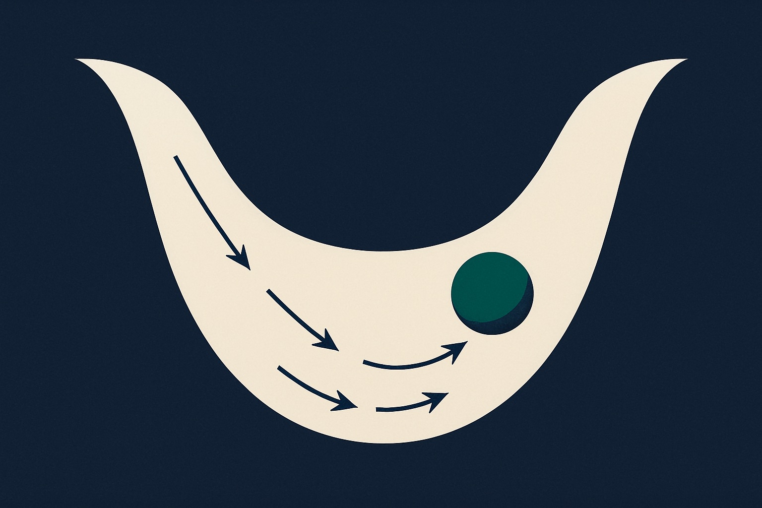
To explain this concept clearly under exam conditions, you should start with a physical analogy before moving to the mathematics. The standard and most accurate analogy is a blindfolded person trying to reach the bottom of a valley. The valley itself represents the cost function, which is often mean squared error for a regression problem or cross-entropy for a classification task. The cost function simply measures how far off our model’s current predictions are from the actual labels in our training data. The coordinates on this landscape represent the weights and biases of our model. Our primary goal is to find the exact combination of weights and biases that results in the lowest possible cost, corresponding to the very bottom of this valley.
Because the person is blindfolded, they cannot look at the whole map to instantly spot the lowest point. This limitation perfectly illustrates why analytical solutions, such as the normal equation, are often computationally impossible for massive datasets or complex deep neural networks. Instead of finding the answer in one step, the algorithm must feel the slope of the ground directly under its feet. In strict mathematical terms, this slope is the partial derivative of the cost function with respect to each individual parameter.
The gradient is a mathematical vector containing all of these partial derivatives. By definition, a gradient points in the direction of the steepest ascent. It tells us exactly which way to step if we wanted to maximise our error. Since our objective is to minimise the error, we take the negative of this gradient. We update our current weights by subtracting a fraction of the gradient, forcing the model to take a step downhill. This iterative process of calculating the slope and taking a step continues until the slope flattens out, indicating we have successfully reached a local minimum.
The mathematical mechanics of a single step
To gain high marks in a written paper, you must be able to demonstrate the exact update rule. For a single weight parameter, the new value is calculated by taking the old value and subtracting the learning rate multiplied by the partial derivative of the cost function with respect to that weight. If the derivative is positive, meaning the cost is increasing as the weight increases, subtracting this positive value naturally reduces the weight. If the derivative is negative, subtracting a negative value increases the weight. In both scenarios, the underlying mathematics correctly forces the parameter toward the minimum cost.
Let us look at a short worked example you might easily encounter in a first-year or second-year paper. Imagine a very simple cost function defined as J(w) = w^2. The derivative of this cost function with respect to the weight w is simply 2w. If our current weight w is 3, our current cost is 9. To find the gradient, we calculate 2 multiplied by 3, which equals 6.
Now we apply the standard update rule. Suppose we have a learning rate of 0.1. We take our current weight of 3 and subtract the product of our learning rate and our gradient (0.1 multiplied by 6). This means we subtract 0.6 from 3, giving us a new weight of 2.4. Our new cost is 2.4 squared, which equals 5.76. We have successfully reduced our cost from 9 to 5.76 in a single mathematical iteration. Showing this step-by-step arithmetic in an exam proves to the examiner that you understand the mechanics behind the abstract formulas.
The crucial role of the learning rate
You cannot explain gradient descent comprehensively without discussing the learning rate, which is usually denoted by the Greek letter alpha. The learning rate is a hyperparameter that controls the exact size of the steps we take during the optimisation process. It acts as a scaling factor applied directly to the gradient before we update our weights. Examiners frequently test your understanding of what happens when you set this value incorrectly, as tuning it is a fundamental part of training practical machine learning models.
If the learning rate is set too small, the algorithm will take tiny, overly cautious steps. While it will eventually reach the minimum, the process will be excruciatingly slow and computationally expensive, potentially taking days to converge on large datasets. Furthermore, in non-convex cost functions like those found in deep learning, a tiny learning rate makes the algorithm highly susceptible to getting permanently trapped in shallow local minima. The model simply cannot build enough momentum to escape these sub-optimal valleys.
Conversely, if the learning rate is too large, the algorithm takes massive steps. It might completely overshoot the minimum of the valley and land on a point much higher than where it started. This causes the gradients to grow even larger on the subsequent iteration, leading to even bigger steps. Very quickly, the cost explodes to infinity, and the model fails to converge entirely. A strong exam answer will explicitly mention this trade-off and might even sketch a quick U-shaped curve showing an oscillating, diverging path to illustrate a learning rate that is set too high.
Differentiating between the main variants
A classic exam question asks you to compare different variants of gradient descent. The version we have discussed so far is technically called Batch Gradient Descent. In the batch variant, the algorithm calculates the error across the entire training dataset before performing a single parameter update. This guarantees a highly stable, consistent path toward the minimum, but it requires loading the entire dataset into active memory. For modern applications containing millions of data points, this approach is entirely impractical.
To solve this memory and computation issue, practitioners use Stochastic Gradient Descent (SGD). Instead of using the whole dataset, SGD calculates the gradient and updates the parameters using only a single training example at a time. This makes the updates incredibly fast, but the path to the minimum becomes very noisy and erratic. Because a single data point might be a statistical outlier, the algorithm might occasionally take steps in the completely wrong direction, zigzagging heavily as it descends the cost landscape.
The industry standard, and the variant you should focus on for application-based questions, is Mini-batch Gradient Descent. This approach takes the best characteristics of both methods. It divides the training data into small batches, typically containing between 32 and 256 examples. The algorithm calculates the gradient over this specific batch and updates the weights accordingly. This provides a much smoother descent than pure SGD while remaining computationally efficient, allowing engineers to train large models on graphics processing units without running out of memory.
How to answer this in an exam
When faced with a 10-mark question asking you to explain gradient descent, structure is everything. Mark schemes heavily reward clear definitions of the cost function and the gradient itself. You will secure the first few marks simply by stating that the gradient points in the direction of steepest ascent and that the algorithm intentionally subtracts it to move downhill.
Next, write out the update equation clearly. Define every single term: the old weight, the learning rate, the partial derivative, and the new weight. Examiners specifically look for the minus sign in the update rule. Omitting this minus sign shows a fundamental misunderstanding of the algorithm’s objective, and you will lose marks immediately.
Finally, include the stopping criteria. How does the algorithm actually know when it is finished? A top-tier answer will state that the process terminates when the gradient approaches zero, meaning the slope has flattened out, or when a predetermined maximum number of iterations has been reached. Demonstrating this complete lifecycle from initialisation to termination is what separates an average student answer from an excellent one.
Frequently Asked Questions
What is the difference between a parameter and a hyperparameter in gradient descent? Parameters are the internal variables the algorithm is actively trying to learn during training, such as the weights and biases of a mathematical model. Hyperparameters are the external settings configured by the user before training begins, such as the learning rate, the batch size, or the maximum number of epochs.
Why do we need partial derivatives instead of normal derivatives? Machine learning models almost always have more than one parameter. Partial derivatives allow us to mathematically isolate how changing one specific weight affects the total cost, assuming all other weights in the network remain entirely constant.
Can gradient descent guarantee finding the global minimum? It can only guarantee finding the global minimum for strictly convex cost functions, like those found in basic linear regression. For the complex, non-convex functions used in deep neural networks, the algorithm is only guaranteed to find a local minimum.
What happens if the starting weights are initialised at zero? In simple linear regression, starting your weights at zero is perfectly fine. However, in neural networks, initialising all weights to zero causes symmetric gradients. This means every neuron in a given layer learns the exact same features, effectively preventing the model from learning any complex patterns.
The Full Marks Press Machine Learning guide covers this entire topic with fully worked exam questions, precise mark scheme breakdowns, and common pitfalls to avoid during your finals. To help you secure top grades in your university modules, you can download a free copy of our revision materials at fullmarkspress.com/free.