Recurrent neural networks vs feedforward networks: key exam differences
The primary difference between a recurrent neural network and a feedforward neural network is how information flows through the architecture. Feedforward networks pass data in one direction from input to output, assuming all input samples are entirely independent of one another. Recurrent networks contain loops that allow information to persist, using a hidden state to maintain a memory of previous inputs to process sequential data.
When you sit your machine learning exam, examiners expect you to understand more than just these basic definitions. You need to articulate why these architectural differences dictate the mathematical limitations and the types of problems each network can actually solve. A feedforward network is the standard architecture you learn first, processing fixed-size vectors to predict a static output. A recurrent network is built specifically for data where the order fundamentally matters, such as natural language processing or financial time-series forecasting. Grasping the distinction between spatial mapping and temporal memory is the foundation of scoring high marks on any neural network architecture question.
Architecture and information flow
A feedforward neural network has a strictly acyclic graph structure. Data enters the input layer, travels through one or more hidden layers, and exits through the output layer. There are absolutely no cycles or loops in this design. The activation of a neuron in a given layer depends exclusively on the outputs from the immediately preceding layer. Because of this linear, one-way street of information, a feedforward network has no concept of time or sequence. If you feed the network the same input vector twice in a row, it will produce the exact same output both times, entirely oblivious to the fact that it just saw that same data a second ago.
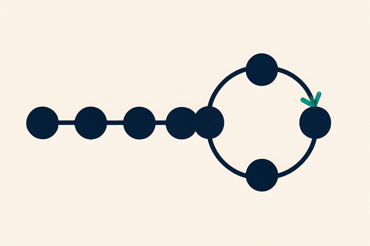
In contrast, a recurrent neural network introduces cycles into its architecture. A neuron in a recurrent network does not just receive input from the current data sample; it also receives input from its own previous state. This cyclic connection creates what we call a hidden state. The hidden state acts as a dynamic memory buffer that updates with every new piece of data the network reads. When the recurrent network processes a sequence, the output at a specific time step is a mathematical function of both the current input and the hidden state from the previous time step.
This architectural distinction means feedforward networks map a single input directly to a single output. Recurrent networks map a sequence of inputs to an output, or even a sequence of inputs to a sequence of outputs. In an exam setting, if a question asks you to draw or evaluate the computation graph of these networks, you must clearly show the directed arrows moving only forward for the feedforward architecture. For the recurrent architecture, you must draw the self-referential loop on the hidden layer and explicitly label the time steps if you are asked to unroll the network on the page.
Handling sequence and time dependencies
The assumption of independence is a massive factor in deciding which network to apply to a dataset. Feedforward networks assume that all data points are independent and identically distributed. Think about a classic task like predicting house prices based on square footage and the number of bedrooms. House A being large has no bearing on House B being small. The network processes each house as a completely isolated event. Furthermore, these networks require fixed-size input vectors. You must specify the exact number of features at the input layer before training begins, and every single sample must match that exact dimension.
Recurrent neural networks discard the independence assumption. They are designed for scenarios where the current data point is highly dependent on the data points that came before it. Take text translation as a concrete example. The meaning of a word in a sentence is heavily context-dependent. If a feedforward network tries to read a sentence word by word, it forgets the beginning of the sentence by the time it reaches the end. A recurrent network carries the context of the early words forward via its hidden state, allowing it to make accurate predictions based on the entire sequence.
Because of this sequential processing, recurrent networks can handle variable-length inputs. A sentence might be five words long or fifty words long. The network simply applies the same computational steps for however many time steps are required. This flexibility makes recurrent architectures the mathematically correct choice for time-series forecasting, speech recognition, and language modelling. In your exam, if a scenario describes data where the order of observations carries meaning, you must justify the use of a recurrent network by referencing its ability to model these temporal dependencies.
Backpropagation vs Backpropagation Through Time
Training these networks requires calculating gradients to update the weights, but the presence of time changes the mathematics entirely. Feedforward networks use standard backpropagation. The algorithm calculates the error at the output layer and propagates it backward through the hidden layers using the chain rule of calculus. Since the network is acyclic, the gradients flow cleanly from the output back to the input in a single, discrete pass.
Recurrent networks require a modified algorithm called Backpropagation Through Time. Because the hidden state at the current time step depends on the hidden state from the previous time step, you cannot just calculate the gradient for the current moment in isolation. You must unroll the network through time, creating a massive, deep feedforward network where each layer represents a specific time step. The error is calculated at the final output and then propagated backward through every single historical time step that contributed to that output.
Let us look at a short worked example of how you might explain this in an exam. Suppose you have a recurrent network processing a sequence of three words to predict a sentiment score. The network reads word one at time step one, word two at time step two, and word three at time step three. To update the weights based on the final prediction error at step three, the algorithm must calculate how the hidden state at step three was affected by the hidden state at step two. Then it must calculate how step two was affected by step one. The final gradient for the weights is the sum of the gradients calculated at each of these sequential steps, relying on a long chain of multiplied derivatives.
This continuous multiplication of derivatives leads directly to the vanishing gradient problem. If the gradients are small fractions, multiplying them together across many time steps causes the final gradient to shrink exponentially until it vanishes completely. The network then fails to learn long-range dependencies because the earliest inputs receive no weight updates. Examiners love asking about this mechanical flaw. You should always link the mechanics of Backpropagation Through Time directly to the vanishing gradient problem when discussing the limitations of standard recurrent networks.
Parameter sharing and network complexity
Another critical difference you must highlight in an exam is how these networks allocate their learnable weights. A feedforward neural network has unique weights for every single connection between layers. If you have an input layer of one hundred neurons and a hidden layer of fifty neurons, there is a distinct weight matrix for that specific transition. If you add more layers, you add completely separate sets of weights. The model capacity grows rapidly with depth, but it means the network must learn the rules of the data independently at every stage of the hierarchy.
Recurrent neural networks employ parameter sharing across time. When a recurrent network is unrolled over fifty time steps, it looks like a fifty-layer feedforward network on paper. However, it does not have fifty different sets of weights. The exact same weight matrices are applied at every single time step. There is one matrix for the input-to-hidden connection, one for the hidden-to-hidden connection, and one for the hidden-to-output connection.
This parameter sharing is highly efficient. It drastically reduces the total number of learnable parameters compared to a fully connected network of similar depth. More importantly, it allows the network to apply the exact same function to the data regardless of where it appears in the sequence. If the network learns to identify a specific grammar pattern at time step two, parameter sharing means it can recognise that exact same pattern if it appears at time step twenty. This translational invariance across time is a massive advantage for sequential data and a key point to raise in exam essays to show a deep understanding of the architecture.
How to answer this in an exam
When faced with a comparative question on these two architectures, mark schemes reward structured, comparative analysis over isolated facts. Do not just list the features of a feedforward network and then list the features of a recurrent network. Instead, compare them directly on specific axes. First, contrast the acyclic architecture with cyclic connections. Second, contrast the assumption of data independence with the modelling of sequential dependencies. Third, contrast standard backpropagation with Backpropagation Through Time, ensuring you mention the unrolling process and parameter sharing.
Finally, examiners look for your ability to select the right tool for a given dataset. If a case study presents patient health records over ten years, state clearly that a recurrent network is required to capture the temporal progression of the disease. If the data is a single snapshot of a patient’s current blood test, a feedforward network is entirely sufficient. The Full Marks Press Neural Networks guide covers this specific type of scenario mapping with worked exam questions, showing you exactly how to structure your answers to hit the top marking bands. Always ground your architectural theory in the practical reality of the data provided in the prompt.
Frequently asked questions
Can a feedforward network handle time-series data at all? Yes, but only if you use a sliding window approach. You can take a fixed number of previous time steps, flatten them into a single input vector, and feed them into a feedforward network. However, this hardcodes the context window size and ignores the true sequential nature of the data, making it far less effective than a recurrent architecture.
Why do recurrent neural networks take longer to train? Recurrent networks are inherently sequential by design. To compute the hidden state at time step ten, the network must first finish computing the states for steps one through nine. This prevents the parallel processing of a single sequence on a GPU, whereas the matrix multiplications in a standard feedforward network can be highly parallelised.
Do Long Short-Term Memory (LSTM) networks count as recurrent networks? Yes, an LSTM is a specific, advanced type of recurrent neural network. It maintains the core cyclic architecture but introduces complex gating mechanisms to the hidden state. These gates mathematically regulate the flow of information, specifically solving the vanishing gradient problem that plagues standard recurrent networks during Backpropagation Through Time.
How do the output layers differ between the two networks? The mathematical function of the output layer is often identical, usually a Softmax function for classification or a linear node for regression. The difference is frequency. A feedforward network produces one output at the end of its forward pass. A recurrent network can produce a single output at the final time step, or it can produce a sequence of outputs by generating a prediction at every single time step.
Get your free exam-revision sample at fullmarkspress.com/free.